Exploring geodata - DAE

the workshop starts here

In this workshop you will install and set up Qgis. We will change some settings and start a project. Then we are ready to add data and explore.

This workshop is made with Qgis version: 3.26.3-Buenos Aires

Preperation

How does this workshop work?

Everytime when you see this: there is a action for you to take on your computer. The text around it is explanation or support. First read a few lines before going to the action points. Sometimes it helps to read further on to better understand what you will be doing.

In the workshop you will find hyperlinks to external resources. Always click with the right mouse button and choose: Open link in a new tab. To not loose the workshop page.

On the right side of the screen you see the contents of the workshop. This also works as a navigation through this page.

What do you need

• A computer
• Internet
• Example data
• Qgis version > 3
• This workshop

Try to work with 2 screens. This way you can have the workshop on 1 screen and Qgis on the other screen (or use a tablet or phone for the workshop).

Preperation

Create a working directory for this workshop, on your computer. In this directory we will place all data and files for this module. During the workshops this will be referred to as 📂 working directory

Download the example data and save it in the 📂 working directory.

Download & install Qgis here

Qgis Documentation

A lot can be found about Qgis online! Please use this. Every tool, feature, term and button can be found and explained in the Qgis documentation.

• Qgis Documentation English v3.28

Setting up Qgis

Open Qgis

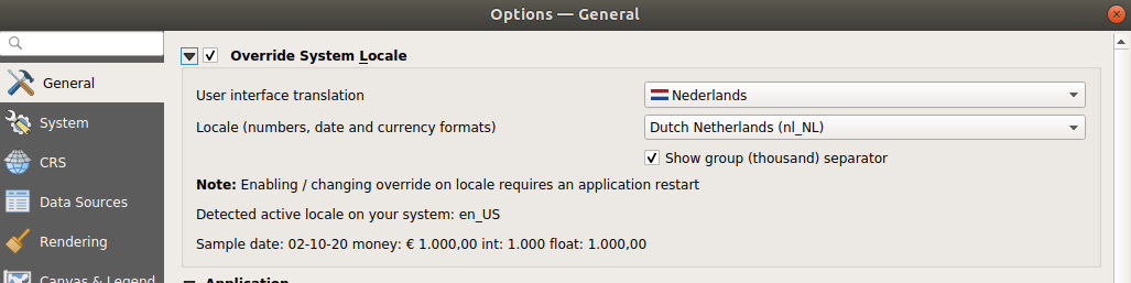
First we will change some basic settings Go to Settings > options and in the panel that opens to General

Here we will change the language to English if it isn’t already so. Qgis sets itself to the language of your system. But for working together it is more convienent to set it to English.

Turn on Override System Locale

Change the language to English

In Options you can also change the icon and text size or the screen theme to dark if you prefer so.

Press Ok and restart Qgis to let the changes take effect.

CRS settings

Let’s immediately set our coordinate reference system (CRS) right. Again go to Settings > options and go to the tab: CRS and Transforms to CRS Handling.

Since our case study is in the Netherlands we want our project to be in RD New of course!

Make sure you set the following settings:

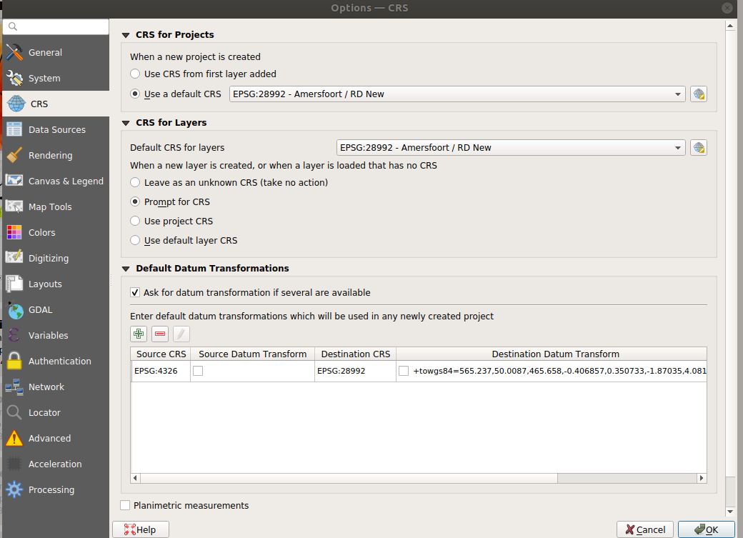
Press Ok when finished.

Panels and Toolbars

The Qgis interface is quite extended, there are a lot of buttons and toolbars. Let’s turn of the things we do not need and turn on the things we do need.

Go to View > Panels and turn on the following panels:

• Browser
• Layers
• Layer Styling

Go to view > Toolbars. Turn of most of them and leave these on:

• Project toolbar
• Selection toolbar
• Map navigation toolbar
• Attributes toolbar
• Manage Layers toolbar

Now we are finished with the basic settings!

Overview of the Qgis interface

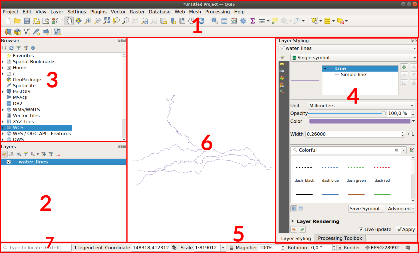
1 Toolbars

2 Layer List

3 Browser

4 Layer Styling Panel

5 Status bar

6 Map canvas

7 Search bar / locator bar

In the Layers panel(2) you will see which data layers you added to your project. The order of the layers is also the order in which the data is displayed on the Map canvas (6). Important is the possibility to toggle on and off the visibility of the layers and the removal of layers. Attention! removing a data layer does not mean you removed the data from your computer. It simply removes the reference and display of the data in the project. Do not be afraid to add and remove layers!

The Status bar(5) shows the current state of the map view. Which coordinate projection you set, the zoom level and scale of the current view. The coordinates of the cursor location. Do you see our project is neatly in RD new (EPSG:28992)?

The Browser (3) is an interesting place to start! Here you have fast access to all the data! Data which is stored on your computer but also all sorts of online services and connections to databases!

The Layer Styling Panel (4) is going to be our best friend. And very convenient to have open at all times. This is were the active layer is styled. It also gets re-rendered immediately so you see the changes in the map view. When working with a lot of data and complicated styles it can be very slow. Turn off the live rendering when working with a lot of data!

Getting data in Qgis

Open a new project

Let’s start. We will start with a empty project.

Go to Project > New

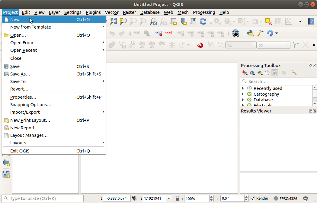
Save this project file in your 📂 working directory and give it a clear file name. Make sure to save regularly Save [Ctrl+S].

Go to Project > Save or Save as..

a Qgis project file The file format of a Qgis Project is .qgs/.qgz. (qgz is the zipped format of gqs) A qgis porject does not contain any data! Only the references to the data and the styling of the data. If you want to share your project with someone else, make sure to share the project file and the data!

Opening data in Qgis

Download the example data and save these in the 📂 working directory.

When storing the data next to the Qgis project in the 📂 working directory then it is really easy to find it in the Qgis browser and open it up.

There are a lot of ways to add data to Qgis.. This can be very confusing. So let’s have a look at the possibilities:

• Through the menu Layer > Add Layer
• The buttons in the Manage Layer toolbar
• Open data from the Browser panel
• Just drag your geo data file from the file browser on your computer into the map view of Qgis. (yes is works too!)

In this workshop we will mostly use the Browser panel

Browser - Project Home

In the Browser panel, ufold the Project Home directory.

This is the folder where the current Qgis project is saved. If you also saved the example data there then we can quickly add them! Can you already see our example datasets?

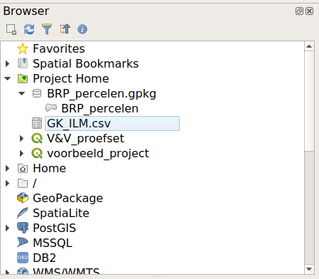
The icon before the file indicates what kind of data it is.

A GeoPackage file is a small sql-lite database, that’s why we see the database icon. If you expand this you see the geo data geometries. For example the BRP-parcels are of the type: polygon.

Open Polygon geometries - BRP parcels and BAG buildings

In our example data is a subset of the BRP dataset, containing crop information on agricultural parcels. Also a subset of the BAG, the building and adres registration dataset. Containing all the buildings and some information of Veenhuizen.

Double click on one of these two files or drag it into the map view.

The layer is now visible in the map view and int he Layers panel!

Because the data and our project is in RDnew EPSG:28992 we do not have to worry about the coordinate reference systems anymore!

BRP Basisregistratie Gewaspercelen

Gewaspercelen bestaat uit de locatie van landbouwpercelen met daaraan gekoppeld het geteelde gewas. De omgrenzingen van de landbouwpercelen zijn gebaseerd op het Agrarisch Areaal Nederland (AAN). De data wordt beheerd door PDOK

Useful vocabulary

Here is a very short list of terms which you may come across when you use QGIS.

Attribute: a piece of data relating to a feature, for example the name of a settlement, or the population > of a region

Attribute table: a table showing the attribute values for all the features in a layer

Buffer: an area of equal distance drawn around a point, line or polygon

Clip: to cut the size of a data object by placing a mask over it - sometimes known as ‘cookie cutter’

Coordinate Reference System (CRS): the system used to reference the x and y coordinates of your data

Feature: an individual object in your data - for example a line, point or polygon

Layer: a set of data, usually of one type which can be turned on and off, moved above or below other > layers, and styled/labelled

Line: vector data which has two ends which don’t meet, possibly with intermediate points - for example > roads or railway lines

Plugin: an optional application which provides additional functionality to QGIS

Point: data comprising sets of individual x and y coordinates, but not joined together - for example > villages or hospitals

Polygon: data comprising one or more closed lines, forming shapes which can be filled - for example land > masses, or provinces

Print Composer: the layout tool within QGIS which is used to produce maps for output

Project: a set of data, styles and Print Composers within QGIS used to make a map

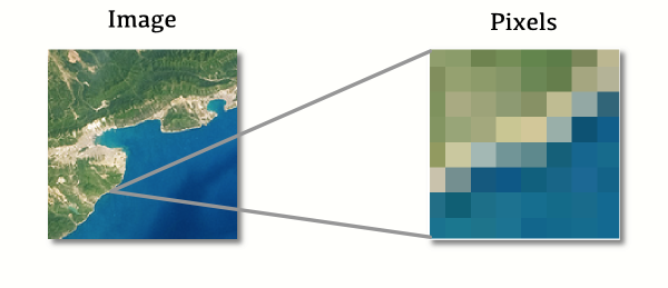
Raster: map data which is represented as an image, with pixel values of between 0 and 255

Style: the rules used to represent data objects with colour, shapes, icons or charts according to the > values of their attributes

Vector: data which is represented as sets of coordinates, producing lines, points or polygons

From: http://antonys.github.io/qgis-workshop/concepts/terms.html

Inspect the data

We now have 2 layers in Qgis. Let’s research what information they contain.

Identify features tool

To quickly find information about the parcels or buildings we can use the Identify features tool. With this tool you can just click on a feature and see the attributes/properties of that specific feature.

Click on the Identify features tool in the top toolbar and then click on a feature on the map.

At the right bottom side of the screen the Identify results panel will appear. Here you can read all the available information about the chosen feature.

Doesn’t it work? Attention! The tool will work on the activated layer from the Layers panel So have a look if you selected the layer. Also in the Identify results panel at the bottom you can choose what mode of information the tool will show you. Now it is set to Current Layer and so will only show information about the chosen active layer.

Attribute table

All the property information of a feature tells us a lot about the dataset. But we can also have a look at this directly.

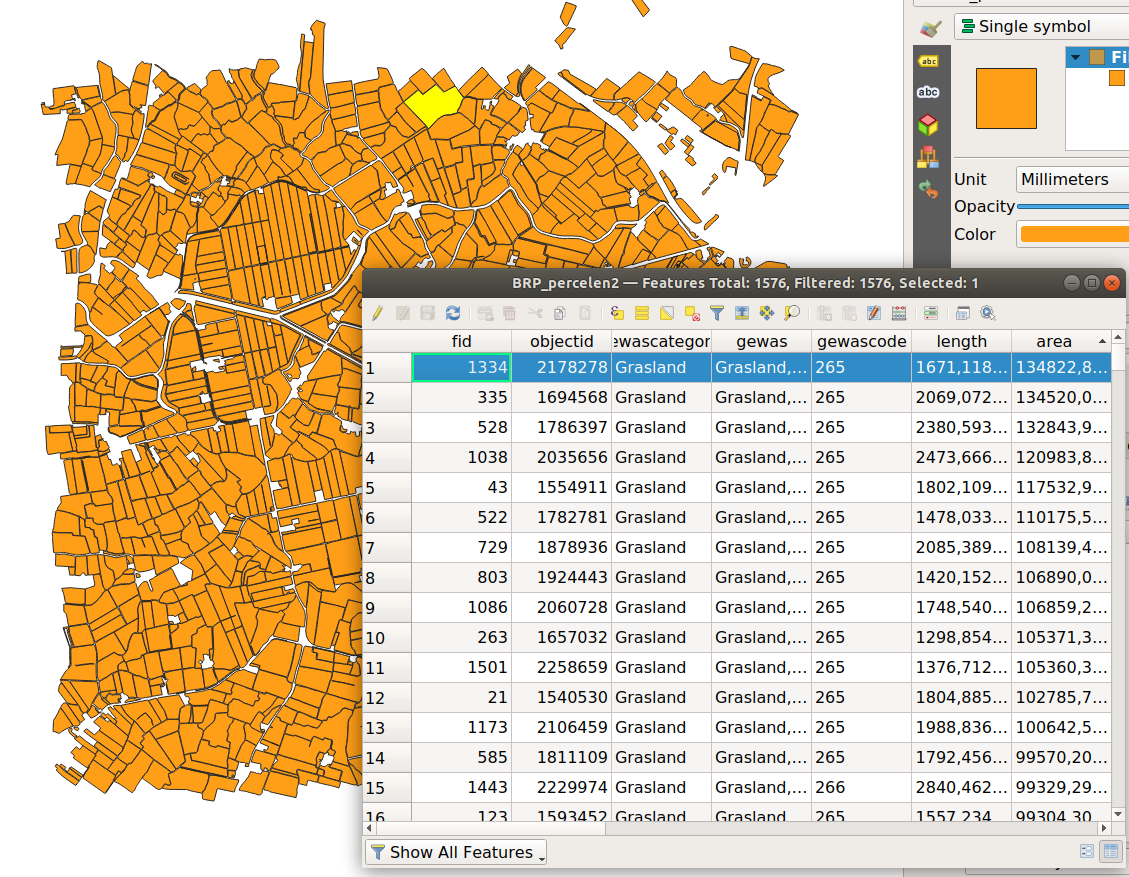
Right click on the BRP parcels layer in the Layers panel and go to Open Attribute Table

Here we again see all the attributes per feature in the dataset. At the top are some selection and navigational buttons.

Sort the attribute data on the size of the parcels. Click on the column header: area. Now the table is organized on the surface size of the parcels! If you click again the order will change. Sort them from large to small.

Select the feature with the largest surface. You do this by clicking on the row number in front of the table, of the chosen feature.

The selected feature will also be highlighted on the map in yellow!

Sometimes it is hard to find your selected feature. Use the buttons at the top of the attribute table to zoom the map to your selected feature. Can you find the buttons?

Now also try to find the smallest parcel.

Remove the selection by pressing:

Also have a look at the attribute table of the building dataset.

Can you find any interesting data?

We are only looking at the data. Selecting and sorting does not change anything to the data itself. So do not be afraid to click around and try some things! .

Close the attribute table.

Properties

Right click on the BRP Parcels layer in the Layers panel, and go to Properties

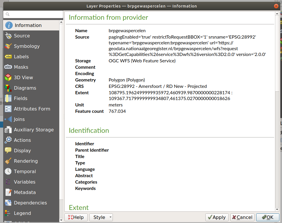
In the tab information you find alle the metadata about this dataset. You can see where it is saved, in which CRS it is and the extent of the dataset.

Can you find how many parcels (features) this dataset contains?

At Source you can find all the settings of the dataset and change them. Although, never just change the CRS here. This is like calling an apple a pear. It stays an apple we just give it another name. If you want to transform the CRS of the data to another one we have to use the Reproject Layer algorithm tool for this.

The Query builder is also interesting, with this we can set some filters on the data.

Fields shows which attribuut fields are present and which data format they contain.

Symbology is for changing the visualization, this is the same as the Layer Styling Panel.

Have a look what other things you can find. For now, these were the most interesting ones.

Close the panel

Visual Data Exploration

Let’s have a look on how to visually explore the data by changing the styling. It is a good habit to first explore a dataset well, so to see if the quality is good, any strange features are present of if we simply have the right data we are looking for!

Make sure the Layer styling Panel is on View > Panels > Layer styling . Move it to the right side of the screen of press F7.

(You can close the Identify Result panel for more space)

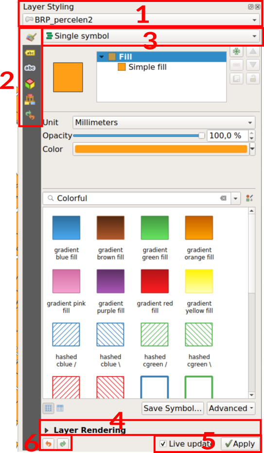
Layer Styling Panel

A brief overview of the panel:

1. Here, we select the layer we are about to style. You can change it here or bij clicking on another layer in the Layers Panel.

2. The available tabs:

   • Styling options
   • Label styling options
   • Masks
   • Symbols
   • Style manager
   • Style history (undo! )

3. Category of feature styling

4. Styling of the whole Layer (Different with feature styling, either separate features or the layer as a whole)

5. Live rendering on and off. If turned on the Apply button is not needed. Turn off when working with really large datasets!

6. Undo/Redo buttons!

Make sure you have the BRP parcels layer active before styling.

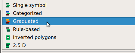
As a default style, a layer has the type simple symbol. Now we will do some data driven styling and style the parcels depending on their area.

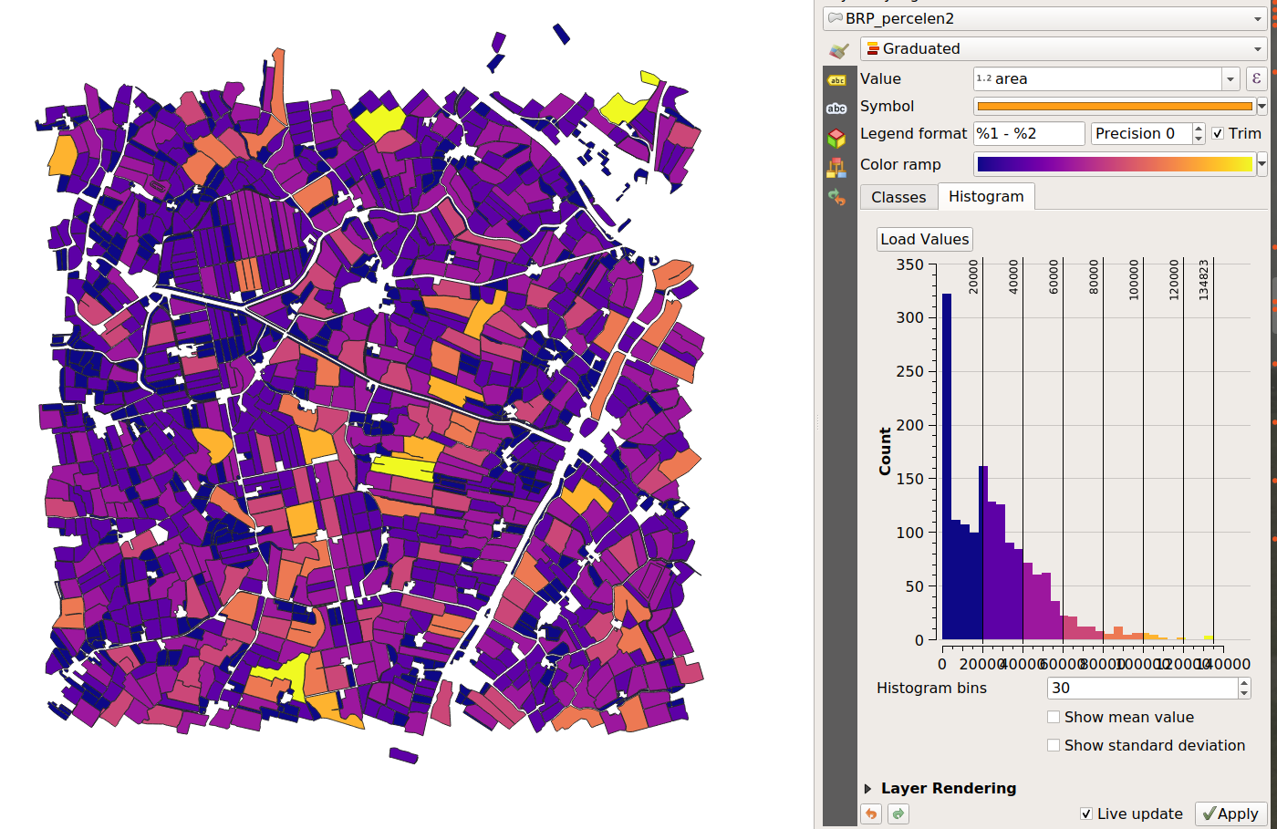
Choose option Graduated because the area is a numeric quantitative variable.

Set value to the attribute: area .

Now click: Classify

Qgis calculates a classification for you. Sometimes the classification is not representative for the data. Therefor, the settings can easily be adjusted and there are a lot of options.

At Classes you can set the amount of classes. At Mode change the classification method.

Set the Mode to Natural Breaks and the amount of classes to 5.

Pick another Color ramp by pressing the dropdown arrow next to the ramp. (right)

Choose the settings that give a good visual insight into the size of the parcels. Can we see the different categories of parcel sizes in Veenhuizen? Can we visually find the largest and smallest parcel?

Also have a look at the Histogram tab. Here you see the data distribution. Put the amount of bins to 50.

Another way to inspect the data is to classify it on crop type!

Change the visualisation to Categorized.

At Value choose : gewas

Click on Classify

Change the Color ramp to Random colors (a continuous color ramp does not suit this type of categorical(nominal) data.

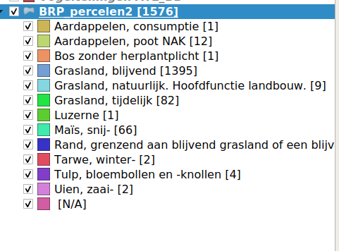
Which crop is the most common in Veenhuizen? Also try sorting on category

Feature count

Left in the Layers panel we see also the legend of our classification. To quickly find how many features per category we have we can turn on the Feature Count.

Richt click on the BRP percelen in the Layers panel, and turn on the Show Feature Count.

Try out some more visualization types and classifications. Also have a look at the buildings. What kind of information can you find?

By changing the visualisation we do not change anything of the data! So do not be afraid to play around with it!

Not happy with your changes? Use the undo and redo buttons at the bottom of the Layer styling panel

Quality

By investigating the data we can also judge the quality of the data a bit. And if the data is relevant for your research.

Please think about:

• Is the data correct? Does this show the environment as it is?
• Did you find out something more that you cannot see in Veenhuizen itself?
• Are the attribuut data values believable of real?
• Did you find any mistakes? What will we do with it?

More data & Plug-ins

There is already a lot of data and maps available on the web. These are made accessible in some plugins. Let’s discover these maps, arial imagery and other datasets!

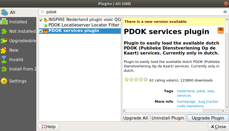
Go to the menu Plugins > Manage and Install Plugins

A new window opens. In the search bar find the next plug-ins and install them with: Install Plugin

• PDOK services
• Quick Map Services
• OSMDownloader
• QuickOSM

After installing the plugins you can close the window. The plugins are available in the menu or in the toolbars. Depending on the plugin were to find them.

Close the window.

PDOK plugin

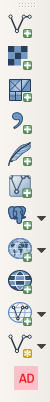
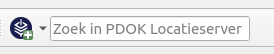
The PDOK plugin comes with a toolbar, which looks like this:

If you do not see it:

Go to the menu View>Toolbars and turn on the PDOK services plugin.

Location server

The search bar of the PDOK toolbar works as a locating service. Here you can search for a place, adres, street etc. in the Netherlands. The map view then zooms and centers to this location.

Type a adres of place name and press enter.

Background maps

The left button on the toolbar brings you to the PDOK services window. All data that PDOK and other Dutch governmental agencies provide can be found here!

Click on the blue PDOK + button on left side of the toolbar.

The window shows you a whole list of available datasets. At the top are the aerial photographic (luchtfoto) images and the standard topographic background maps (achtergrondkaart).

Click on the Luchtfoto Actueel Ortho 8cm RGB. To add it to the map, double click on it or choose on of the buttons at the bottom : Standaard, Boven (top) or Onder (bottom).

Also add some background maps: standaard | WMTS | BRT achtergrondkaart

I can’t see the layers? Layer order

In the Layers panel, the visual order of the layers is determined and can be changed. The layer at the top of the list will also be visualized on top. The data underneath will not be visible then. Just drag the layers into a good order in the panel.

Available data

In the PDOK services is also a lot of data to be found. At the top is a search bar.

Search for : natura2000

About natura 2000 areas

There are multiple datasets available. Make sure you choose the natura 2000 of the type WFS service.

Add this layer to the map view and close the panel.

Can you find the peat location to the south of Veenhuizen?

Use the Identify Features tool to click on the area. What kind of attribute data is available? What is the name of this area?

Again search in the PDOK services for : bodemkaart (soil map) and add the layer Bodemvlakken - WMS - BRO Bodemkaart (soil information)

Again use the Identify Features tool to click on a area. What kind of attribute data is available?

• Did you notice the difference in data types between the natura areas and the bodemkaart?
• What kind of difference is there?

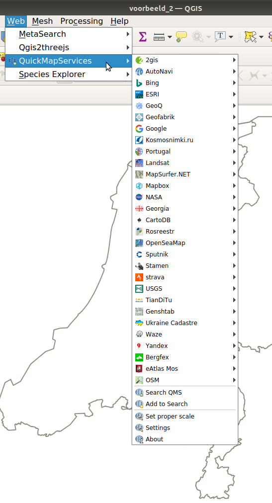
Quick Map Services

QuickMapServices is a plug-in which provides different background maps to use as a reference in your project. Mostly international world covering maps. They do not contain any data. But do provide good background references!

Go to the menu web > Quick map services

There are a few providers in the list, but there are way more! Let’s add these first.

Go to the Settings of the QuickMapServices (at the bottom in the sub menu)

Go to the tab: More Services

Click on get contributed pack

Accept and Save. close the Settings window.

Again go to the menu web > Quick map services

We have a lot more background maps available.

Add a map which seems interesting to you. Have a look around.

Also a tutorial here: https://docs.qgis.org/3.28/en/docs/training_manual/qgis_plugins/plugin_examples.html

Quick OSM downloads plugin

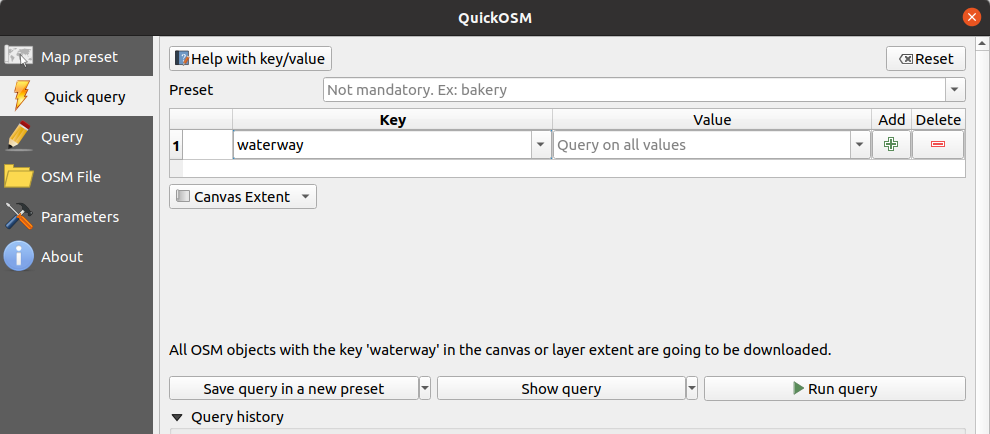
Follow this tutorial for the QuickOSM plugin:

https://docs.qgis.org/3.28/en/docs/training_manual/qgis_plugins/plugin_examples.html

Instead of railway we will add the waterway

And choose Canvas extent instead of Layer extent